Too easy! WTF?#

Parameters and Deterministic Properties#

TODO

Graph Diameter#

For a graph $G = (V, E)$, the eccentricity of a vertex $v \in V$ is the maximum distance between $v$ and another vertex, i.e., essentially the height of the BFS-tree rooted in $v$. The diameter of $G$ is the largest eccentricity over all vertices.

A vertex with minimum eccentricity 2, one with maximum
eccentricity 4, and the corresponding diameter path of length 4. — page 1 — A vertex with minimum eccentricity 2, one with maximum eccentricity 4, and the corresponding diameter path of length 4.

A vertex with minimum eccentricity 2, one with maximum
eccentricity 4, and the corresponding diameter path of length 4. — page 2 — A vertex with minimum eccentricity 2, one with maximum eccentricity 4, and the corresponding diameter path of length 4.

It’s Hard#

The diameter can be trivially computed by running a BFS from every vertex, yielding running time $O(nm)$. For sparse graphs, this is the best we can do: under OV, there is no $O(n^{2 - \varepsilon})$ algorithm that distinguishes between diameter 2 or 3 in sparse graphs [3, 4].

Typical Inputs#

It is probably fair to say that real-world networks are an important type of input for computing the diameter.

There are probably other applications where computing the diameter appears as a subproblem. It would be nice to have a collection of instances coming from such applications.

Too Easy!#

There are actually multiple diameter algorithms that are way too fast. To name two examples:

BoundingDiameters runs a BFS from only 21 vertices to compute the diameter of the social network hyves with 8 M vertices and 871 M edges [5].
iFUB runs a BFS from only 7 vertices to compute the diameter of the computer network as-skitter with 1.7 M vertices and 22 M edges [6].

iFUB#

The iFUB algorithm [6] first computes a central vertex $c$ that (hopefully) has low eccentricity. Afterwards it runs a BFS from all vertices that are far away from the center $c$. Assume we have run the BFS for every vertex with distance at greater than $d$. Then any future BFS from the remaining vertices can only yield new paths of length at most $2d$, as we can always go via the vertex $c$. Thus, if we have already found a shortest path of length $2d$, we can stop.

Vertex $v$ has eccentricity $2d$.
Between any two vertices in the blue region, the distance is at most
$2d$. Thus, if we have done a BFS form every vertex outside the blue
region, we have found the diameter. — page 1 — Vertex $v$ has eccentricity $2d$. Between any two vertices in the blue region, the distance is at most $2d$. Thus, if we have done a BFS form every vertex outside the blue region, we have found the diameter.

There are different heuristics to find a central vertex.

max degree

Choose a vertex of maximum degree.

double sweep

Start with an arbitrary vertex $u$ chooses a vertex $v$ at maximum distance, with the idea that $v$ is at the “periphery” of the graph. As central vertex, choose a vertex $w$ that is in the middle layer of the BFS tree of $v$.

4-sweep

Run two double sweeps, starting the second double sweep with the result of the first double sweep. One can also start the first double sweep with a vertex of maximum degree.

BoundingDiameters#

BoundingDiameters [5] makes use of the following observation. Running a BFS from one vertex to compute its eccentricity also lets us learn something about the eccentricity of other vertices. Specifically, if two vertices $u$ and $v$ have distance $d$, then their eccentricities differ by at most $d$.

Running a BFS from $v$
tells us not only that $v$'s eccentricity is $4$, but also that $u$
and $w$ have eccentricity between $3$ and $5$. — page 1 — Running a BFS from $v$ tells us not only that $v$’s eccentricity is $4$, but also that $u$ and $w$ have eccentricity between $3$ and $5$.

This yields lower and upper bounds for the eccentricities, which in turn yield lower and upper bounds for the diameter. The algorithm BoundingDiameters essentially tries to pick a small set of root vertices $R \subseteq V$, such that running a BFS from each root suffices to know the exact diameter. This is done by iteratively adding vertices to $R$. A vertex $v$ is excluded from being added to $R$ if:

the lower and upper eccentricity bound for $v \in V$ coincide or
improving the eccentricity bound of $v$ can no longer improve the diameter bound (e.g., its eccentricity is known to be smaller than the diameter).

The search is stopped, if:

there are no root-candidates left or
the upper and lower bound for the diamter coincide.

There are different strategies for selecting the next root [5]. Alternating between vertices with small lower bound and vertices with high upper bond on their eccentricity is most successful.

SumSweep#

The SumSweep algorithm [13] is similar to BoundingDiameters but works for arbitrary directed graphs. The core differences come from dealing with the graph being directed, e.g., the algorithm maintains a forward and backward eccentricity and for each root a forward and backward BFS are performed.

It is probably fair to view SumSweep as an extension of BoundingDiameters and to assume that insights for the former likely translate to the latter.

WTF?#

There are multiple approaches attempting to explain the good performance, together yielding a decent understanding.

Locality and Heterogeneity#

The experiments in [1] study how many BFS runs iFUB requires depending on locality and heterogeneity, comparing generated graphs with real-world networks.

Locality, heterogeneity, and graph models.

The locality of a graph measures how distant the endpoints of an edge are in the rest of the graph. Think of high locality as: the graph has an underlying geometry, it has many triangles, there is a high dependence between the edges.

The heterogeneity of a graph describes the variance of the degree distribution. Road networks are homogeneous with all vertices having roughly the same degree. Social networks tend to be heterogeneous with low average degree and a heavy tail of few high-degree vertices (think power-law).

The experiment setup in [1] is roughly as follows. Generate graphs with varying locality and heterogeneity (and constant average degree). Locality is achieved with an underlying geometry. Heterogeneity is achieved with connection probabilities depending on vertex weights. This essentially provides a clean lab-environment, where one can observe how the running time of algorithms changes depending on locality and heterogeneity in isolation from other graph properties. These experiments on generated graphs are complemented and compared with experiments on a large number of real-world networks from different domains.

Insight#

On inputs that have locality or a heterogeneous degree distribution (or both), we can expect iFUB with 4-sweep to be fast. Notable exception: Graphs with an underlying geometry that wraps around (e.g., sphere or torus).

Explanatory Power#

The empirical observations paint a coherent picture.

One can observe a clear dependence on locality and heterogeneity that is consistent between generated and real-world networks.

Changing the heuristic that selects the central vertex consistently impacts the running time for different graphs between generated and real-world networks.

For homogeneous graphs with geometry, the models predict good performance unless the geometry wraps around (sphere, torus, etc.). Visualizations of real-world graphs with matching properties and bad performance show wrapping geometry.

Limitations#

These are only experiments, not proofs.

The number of BFS runs has high variance, even for the model when generating multiple graphs with the same parameter. This indicates that a theoretical analysis on the model might be difficult and that the properties locality and heterogeneity do not fully capture the running time behavior.

Random Geometric Graphs#

In [14], there is an analysis of iFUB on random geometric graphs (RGG). RGGs are usually obtained by placing vertices at random positions in the unit square and connecting vertices that are close. Alternatively, a torus RGG is generated by using the flat torus instead (i.e., unit square with opposite sides identified).

Insight#

On random geometric graphs with average degree $n^x$, iFUB with double sweep runs a BFS from $\tilde O(n^{1 - \frac{2}{3}x})$ vertices. On torus RGGs, it requires $\Omega(n)$ BFS runs.

Explanatory Power#

The theoretical result matches the general trend of the empirical observations: RGGs are prototypical for homogeneous graphs with locality, which should result in a low running time, unless the geometry wraps around.

Limitations#

The upper bounds are very far from matching empirical performance. It in particular makes no statement about sparse graphs.

Power-Law Graphs#

One can obtain strong performance bounds for iFUB and SumSweep by assuming four (rather technical) properties that I would summarize as follows [20]:

The size of the BFS layers for different vertices of the same degree grows at a similar rate.
Let $A \subseteq V$ and $B \subseteq V$ be the $i$-th and $j$-th layer of a BFS from $s \in V$ and $t \in V$, respectively. If $|A| \cdot |B| \ge n^{1 + \varepsilon}$, then $\mathrm{dist}(s, t) \le i + j$, i.e., the BFS search spaces from $s$ and $t$ have met after $i$ respectively $j$ steps.
The search spaces in property 2 rarely meet much earlier.
The degree distribution follows a power law.

Properties 2 and 3 can in a sense be viewed as requiring sufficient stochastic independence between edges such that the birthday paradox can be applied: An edge between $A$ and $B$ is likely if and only if there are enough pairs of vertices in $A \times B$ that could form an edge.

Insight#

On graphs satisfying properties 1 – 4 (power-law degree distribution, stochastic independence of edges, uniform search-space growth), iFUB and SumSweep run in almost linear time.

Explanatory Power#

The almost linear upper bounds are quite strong and fit well to the empirical observations.

The deterministic properties make it so that the results are not specific to just one probabilistic network model.

The authors provide experiments that aim to validate the properties for real-world networks.

Limitations#

The results are restricted to graphs with a power-law degree distribution and logarithmic diameter.

Many real-world networks have strong dependence between edges. Properties 2 and 3 requiring enough independence to apply the birthday paradox seem questionable in this context.

The properties are very complicated. Also see the discussion on deterministic properties.

The properties are difficult to check:

They involve asymptotics using big O notation, which is not meaningful for individual inputs.

Statements on search-space growth are difficult to check when there are only few steps due to a logarithmic diameter.

Small Certificates#

The efficiency of BoundingDiameters and iFUB is based on the existence of a small diameter certificate: a small set of vertices $X \subseteq V$ such that knowing the distance from every vertex in $x$ to all other vertices provides matching upper and lower bounds for the diameter. With this, one can ask these two questions:

Why do many practical inputs have a small diameter certificates?
If there is a small diameter certificate, why can it be found efficiently?

Question 2 is answered positively by [21]:

Insight#

If there is a truly sublinear diameter certificate, then there is a truly subquadratic randomized algorithm finding it.

Explanatory Power#

The considered certificates fit to those found by algorithms that are efficient in practice.

There are several graphs classes that have small diameter certificates [21]. This to some degree also answers question 1 of why many inputs have small certificates.

Limitations#

For constant certificates, the running time is still $O(m \sqrt{n})$, which is quite pessimistic.

While this provides an algorithm that finds a small certificate (somewhat) efficiently, this does not explain why the specific strategies of BoundingDiameters or iFUB find it efficiently.

One could argue that this parameter (size of a diameter certificate) is quite close to the running time; see the discussion on deterministic properties.

References#

On the External Validity of Average-case Analyses of Graph Algorithms by Thomas Bläsius, Philipp Fischbeck (2023)
Fast approximation algorithms for the diameter and radius of sparse graphs by Liam Roditty, Virginia Vassilevska Williams (2013)
Towards Sub-Quadratic Diameter Computation in Geometric Intersection Graphs by Karl Bringmann, ‪Sándor Kisfaludi-Bak, Marvin Künnemann, André Nusser, Zahra Parsaeian (2022)
Determining the diameter of small world networks by Frank W. Takes, Walter A. Kosters (2011)
On computing the diameter of real-world undirected graphs by Pilu Crescenzi, Roberto Grossi, Michel Habib, L. Lanzi, Andrea Marino (2012)
Fast diameter and radius BFS-based computation in (weakly connected) real-world graphs by Michele Borassi, Pierluigi Crescenzi, Michel Habib, Walter A. Kosters, Andrea Marino, Frank W. Takes (2015)
Diameter Computation on (Random) Geometric Graphs by Thomas Bläsius, Annemarie Schaub, Marcus Wilhelm (2026)
An Axiomatic and an Average-Case Analysis of Algorithms and Heuristics for Metric Properties of Graphs by Michele Borassi, Pierluigi Crescenzi, Luca Trevisan (2017)
Certificates in P and Subquadratic-Time Computation of Radius, Diameter, and all Eccentricities in Graphs by Feodor F. Dragan, Guillaume Ducoffe, Michel Habib, Laurent Viennot (2025)

Clique Enumeration#

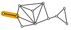
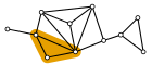
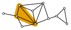
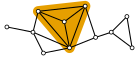
A clique in a graph is a fully connected subgraph. It is maximal if it is not contained in a larger clique. The goal of clique enumeration is to compute a list of all maximal cliques of a given graph.

Example of enumerating all
maximal cliques. — page 1 — Example of enumerating all maximal cliques.

Example of enumerating all
maximal cliques. — page 2 — Example of enumerating all maximal cliques.

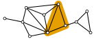
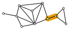
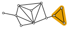
Note that the problem is equivalent to enumerating maximal independent sets on the complement graph.

It’s Hard#

The number of maximal cliques $\alpha$ of a graph can be exponential. When removing the edges of $\frac{n}{3}$ disjoint triangles from the complete graph $K_n$ ($n$ divisible by $3$), then one obtains a maximal clique by selecting exactly one vertex for each of the $\frac{n}{3}$ triangles, yielding $\alpha = 3^{n / 3} \approx 1.44^n$ maximal cliques. This bound is tight [7].

One can enumerate all maximal cliques in $O(3^{n / 3})$ time [8]. This is worst-case optimal as it matches the above bound. Thus, one cannot get better bounds that only depend on the input size. When considering dependence on the output size $\alpha$, the best known bounds are:

$\alpha \cdot O(n \bar{m})$ [9] ($\bar{m}$: number of edges in the complement)
$\alpha \cdot O(n m)$ [10] (using that graphs have arboricity $O(n)$)
$\alpha \cdot O(n^{2.094})$ [11] ($2.094$ comes from rectangular matrix multiplication)

All three bounds are delay bounds, i.e., the time between outputting solutions is in $O(n \bar{m})$, $O(n m)$, and $O(n^{2.094})$, respectively.

Typical Inputs#

It is probably fair to say that real-world networks are an important type of input for enumerating cliques.

There are probably other applications or problems where it could be useful to know all maximal cliques. It would be nice to have a collection of instances coming from such applications.

Too Easy!#

The algorithm in [12] only needs seconds to enumerate all cliques of graphs millions of vertices and edges. Here are just two examples:

On the network web-Google with 875 k vertices and 4.3 M edges, all 1.4 M maximal cliques are enumerated in under 10 s.
On the network cit-Patents with 3.8 M vertices and 16.5 M edges, all 14.8 M maximal cliques are enumerated in under 30 s.

Observe that the number of cliques in these examples is far from being exponential. In fact, there are less maximal cliques than edges in both cases. These are not outliers. In experiments on 2740 real-world networks, the vast majority of 2552 networks have at most $m$ maximal cliques [1], while only 188 networks have more maximal cliques than edges.

But even given that the number of maximal cliques is so low, worst-case bounds of $O(nm)$ or $O(n^{2.094})$ per clique are way to pessimistic.

WTF?#

The paper [12] is actually great in that in not only provides the practically highly efficient algorithm but also a tight parameterized analysis. See the discussion for parameterized results below.

Parameterized by Sparsity#

Multiple parameters have been considered, all in some way related to sparsity. For a better overview, here a list of parameters used in the following:

symbol	parameter
$n$	number of vertices
$m$	number of edges
$\alpha$	number of maximal cliques
$\omega$	size of largest clique
$\Delta$	maximum degree
$a$	arboricity The minimum number of forests into which the edges can be partitioned.
$d$	degeneracy The minimum number $d$ such that every subgraph has maximum degree at most $d$. In other words, there is an order of vertices such that deleting the vertices in this order never deletes a vertex with degree larger than $d$.
$c$	weak closure The closure captures the property that vertices with many common neighbors are connected. Formally, call a vertex $v$ is $c$-deletable if there is no non-adjacent vertex $u$ that has at least $c$ common neighbors with $v$. A graph is weakly $c$-closed if exhaustively deleting $c$-deletable vertices results in the empty graph. The weak closure $c$ is the minimum number for which the graph is weakly $c$-closed.

The following table shows results on parameterized enumeration times. The note “delay” means that if the enumeration is $\alpha\cdot T$, then at most $T$ time elapses between outputting two solutions.

enumeration time	note	paper
$O(dn 3^{d / 3})$	$\alpha \le (n - d) 3^{d / 3}$	[12]
$\alpha \cdot O(\mathrm{poly}(d))$		[15]
$\alpha \cdot O(n \mathrm{poly}(c))$	$\alpha \le 3^{(c - 1)/3} n^2$	[16, 17]
$\alpha \cdot O(am)$	delay	[10]
$\alpha \cdot O(\Delta^4)$	delay	[18]
$\alpha \cdot \tilde O(\omega d(\Delta + \omega d))$	delay	[19]
$\alpha \cdot O(\min\{md, \omega d\Delta\})$	delay	[19]

There is probably a lot to say for each individual result. To keep it non-repetitive, I’ll focus on the degeneracy bound in [12] (which seems most relevant as the algorithm is highly efficient in practice) and discuss the other bounds where interesting.

Insight#

Enumerating cliques is fast on sparse graphs.

Explanatory power#

I think this already provides a rather good high-level explanation for the good performance in practice. Here are some highlights:

Good upper bound for specifically the algorithm that is fast in practice [12].

Multiple of the papers check whether the considered are reasonably small in real-world networks.

For the 188 networks in [1] that have more than $m$ cliques, there is a strong positive correlation between the degeneracy and the number of cliques. The bound in [12] seems to be a great fit here.

Limitations#

Experiments with 2740 real-world networks [1] show that the density-explanation (while fitting for 188 networks) is not satisfying for the vast majority of 2552 networks that have less than $m$ cliques:

The exponential upper bound with respect to the degeneracy is too pessimistic to explain less than $m$ maximal cliques.

There is no (or in fact slight negative) correlation with the degeneracy.

There is a strong correlation with locality, i.e., graphs with high locality tend to have fewer maximal cliques (more details).

While the weak closure $c$ in theory captures the concept of locality, there is no correlation. In practice, the weak closure and degeneracy are essentially the same, with degeneracy being usually only a small factor larger than $c - 1$.

Even accepting that the number of maximal cliques $\alpha$ is very small, does not explain enumerating 1.4 M and 14.8 M cliques in under 10 s and 30 s, respectively:

The bound in [12] is not output-sensitive, unless $\alpha$ matches the upper bound, which is exponential in $d$.

The other bounds have rather high cost per clique. The bound of $O(\mathrm{poly}(d))$ per clique [15] is the most reasonable but still too pessimistic for the practical observations.

Probabilistic Network Models#

The experiments in [1] study the number of maximal cliques depending on locality and heterogeneity, comparing generated graphs with real-world networks.

Locality, heterogeneity, and graph models.

Insight#

We can expect sparse graphs to have at most $m$ maximal cliques. The exact number depends on the locality: Graphs without locality have close to $m$ maximal cliques and this number shrinks with increasing locality.

The above insight is purely based on experiments [1]. There is also a theoretical analysis for hyperbolic random graphs [22] and geometric inhomogeneous random graphs [23]; network models with locality and heterogeneity. We note that these theoretical bounds for the models seem to disagree with the previous experiments on the same models.

Insight#

We can expect graphs with graphs locality and a heterogeneous degree distribution to have a super-polynomial number of maximal cliques.

Explanatory Power#

The models fit exceptionally well to the large majority of 2552 out of 2740 real-world networks:

They consistently have at most $m$ maximal cliques.

When representing the number of maximal cliques as $\alpha = x \cdot m$, then even the value of $x$ (which decreases for increasing locality) is consistent between the models and the real-world networks.

Limitations#

This can only explain the number of maximal cliques. It does not explain why the algorithm does also find them efficiently.

There are still the remaining 188 real-world networks, with different behavior. We do not know the difference between them.

Asymptotics are broken here: While the models agree with the real world in experiments, the asymptotic analysis seems to contradict these observations. The reason for this is that the super-polynomial growth only supersedes the linear terms for really large graphs.

References#

On the External Validity of Average-case Analyses of Graph Algorithms by Thomas Bläsius, Philipp Fischbeck (2023)
On cliques in graphs by J. W. Moon, Leo Moser (1965)
The worst-case time complexity for generating all maximal cliques and computational experiments by Etsuji Tomita, Akira Tanaka, Haruhisa Takahashi (2006)
A New Algorithm for Generating All the Maximal Independent Sets by Shuji Tsukiyama, Mikio Ide, Hiromu Ariyoshi, Isao Shirakawa (1977)
Arboricity and Subgraph Listing Algorithms by Norishige Chiba, Takao Nishizeki (1985)
An Improved Upper Bound on Maximal Clique Listing via Rectangular Fast Matrix Multiplication by Carlo Comin, Roméo Rizzi (2018)
Listing All Maximal Cliques in Large Sparse Real-World Graphs by David Eppstein, Maarten Löffler, Darren Strash (2013)
A new decomposition technique for maximal clique enumeration for sparse graphs by George Manoussakis (2018)
Finding Cliques in Social Networks: A New Distribution-Free Model by Jacob Fox, Tim Roughgarden, C. Seshadhri, Fan Wei, Nicole Wein (2020)
Efficient maximal cliques enumeration in weakly closed graphs by George Manoussakis (2023)
New Algorithms for Enumerating All Maximal Cliques by Kazuhisa Makino, Takeaki Uno (2004)
Sublinear-Space and Bounded-Delay Algorithms for Maximal Clique Enumeration in Graphs by Alessio Conte, Roberto Grossi, Andrea Marino, Luca Versari (2019)
On the Number of Maximal Cliques in Two-Dimensional Random Geometric Graphs: Euclidean and Hyperbolic by Hodaka Yamaji (2023)
Maximal cliques in scale-free random graphs by Thomas Bläsius, Maximilian Katzmann, Clara Stegehuis (2024)

Real-World Networks#

The term real-world networks describes graphs that are the direct representation of a relation existing in the real world. Examples are friendships between persons (social network), collaborations between researchers (collaboration network), roads between intersections (road networks), cables between autonomous systems forming the internet (technical networks), or interactions between proteins (biological networks).

Problem Instances#

Real-world networks are an important type of input for many graph problems. A nice collection of networks used in [1] can be found on Zenodo [2]. Additional networks are available via Network Repository, KONECT, and SNAP.

Limitations#

Graph algorithms have applications that go beyond computing some property on a real-world network. In these cases, the input graph is often some kind of auxiliary graph, which might have very different properties than typical real-world networks.

It clearly depends on the specific problem whether real-world networks can be seen as “practical inputs”. While computing the diameter is important when studying real-world networks, computing a large independent set is probably more relevant for auxiliary graphs modeling some kind of conflicts (e.g., when computing a maximum number of non-overlapping labels on a map).

While a large collection of real-world networks is readily available, the situation is less stellar for other types of inputs. We should probably try to change that.

References#

On the External Validity of Average-case Analyses of Graph Algorithms by Thomas Bläsius, Philipp Fischbeck (2023)
almost 3000 Networks (unweighted, undirected, simple, connected) from Network Repository by Thomas Bläsius, Philipp Fischbeck (2023)

References#

On the External Validity of Average-case Analyses of Graph Algorithms by Thomas Bläsius, Philipp Fischbeck (2023)
almost 3000 Networks (unweighted, undirected, simple, connected) from Network Repository by Thomas Bläsius, Philipp Fischbeck (2023)
Fast approximation algorithms for the diameter and radius of sparse graphs by Liam Roditty, Virginia Vassilevska Williams (2013)
Towards Sub-Quadratic Diameter Computation in Geometric Intersection Graphs by Karl Bringmann, ‪Sándor Kisfaludi-Bak, Marvin Künnemann, André Nusser, Zahra Parsaeian (2022)
Determining the diameter of small world networks by Frank W. Takes, Walter A. Kosters (2011)
On computing the diameter of real-world undirected graphs by Pilu Crescenzi, Roberto Grossi, Michel Habib, L. Lanzi, Andrea Marino (2012)
On cliques in graphs by J. W. Moon, Leo Moser (1965)
The worst-case time complexity for generating all maximal cliques and computational experiments by Etsuji Tomita, Akira Tanaka, Haruhisa Takahashi (2006)
A New Algorithm for Generating All the Maximal Independent Sets by Shuji Tsukiyama, Mikio Ide, Hiromu Ariyoshi, Isao Shirakawa (1977)
Arboricity and Subgraph Listing Algorithms by Norishige Chiba, Takao Nishizeki (1985)
An Improved Upper Bound on Maximal Clique Listing via Rectangular Fast Matrix Multiplication by Carlo Comin, Roméo Rizzi (2018)
Listing All Maximal Cliques in Large Sparse Real-World Graphs by David Eppstein, Maarten Löffler, Darren Strash (2013)
Fast diameter and radius BFS-based computation in (weakly connected) real-world graphs by Michele Borassi, Pierluigi Crescenzi, Michel Habib, Walter A. Kosters, Andrea Marino, Frank W. Takes (2015)
Diameter Computation on (Random) Geometric Graphs by Thomas Bläsius, Annemarie Schaub, Marcus Wilhelm (2026)
A new decomposition technique for maximal clique enumeration for sparse graphs by George Manoussakis (2018)
Finding Cliques in Social Networks: A New Distribution-Free Model by Jacob Fox, Tim Roughgarden, C. Seshadhri, Fan Wei, Nicole Wein (2020)
Efficient maximal cliques enumeration in weakly closed graphs by George Manoussakis (2023)
New Algorithms for Enumerating All Maximal Cliques by Kazuhisa Makino, Takeaki Uno (2004)
Sublinear-Space and Bounded-Delay Algorithms for Maximal Clique Enumeration in Graphs by Alessio Conte, Roberto Grossi, Andrea Marino, Luca Versari (2019)
An Axiomatic and an Average-Case Analysis of Algorithms and Heuristics for Metric Properties of Graphs by Michele Borassi, Pierluigi Crescenzi, Luca Trevisan (2017)
Certificates in P and Subquadratic-Time Computation of Radius, Diameter, and all Eccentricities in Graphs by Feodor F. Dragan, Guillaume Ducoffe, Michel Habib, Laurent Viennot (2025)
On the Number of Maximal Cliques in Two-Dimensional Random Geometric Graphs: Euclidean and Hyperbolic by Hodaka Yamaji (2023)
Maximal cliques in scale-free random graphs by Thomas Bläsius, Maximilian Katzmann, Clara Stegehuis (2024)